- ✓ No installation required
- ✓ No Microsoft Excel or Office needed
- ✓ Works in any modern browser
- ✓ Cross-platform: Windows, Mac, Linux, mobile
- ✓ Upload Excel or CSV and analyze instantly
💻 Use with Excel
- ✓ Offline processing, no internet needed
- ✓ Requires Windows + Excel 2016 or higher
- ✓ Microsoft 365 recommended
- ✓ Faster for very large datasets
- ✓ 100% local — data never leaves your device
The step-by-step instructions below use the Desktop Version (Use with Excel) as the example. The Web Version (Use Online) follows the same analytical workflow — simply upload your file in the browser to get started.
The following instructions use a "Electronics Stores" virtual dataset to demonstrate how to use the WaterfallBridge tool to automatically generate Bridge analysis and identify key driving factors.
📋 Before you begin, make sure your data is in the right format. Read the Data Preparation Guide →
1–5. Step-by-Step Instructions
Show the step-by-step manual walkthrough
The initial panel displays two buttons: "New Bridge File" and "Open Existing Bridge File"

1.1 Click "New Bridge File" button - Generates a new Excel file containing a new "Data" worksheet. Please enter the corresponding data in the "Data" worksheet for further analysis.
1.2 Click "Open Existing Bridge File" button - Select a previously used Excel file. This file should contain the relevant data and have Data Types configured.
In the Data worksheet starting from column B, enter data types in the first row, field names in the second row, and data in all rows from the third row onwards. Column A contains auto-generated identifiers for the first three rows that need data input. Column A itself has no impact on data and analysis.

In the first row of the "Data" worksheet, use the generated dropdown menu starting from column B to select the data type. The type depends on the meaning the data needs to represent. The program will automatically analyze based on the data type.
Data types are divided into 5 categories: Dimension, Key, SumY, SumN, Result. Each field must be defined with one data type, which can be selected using the dropdown menu.

Now using our simulated supermarket data as an example, let's explain the meaning of each data type. Each type is defined as follows:

For example: If "Product Name" is selected as Key, the tool will calculate the impact of each variable's change on the final result (Result) within this "Product Name" dimension.

For example: Quantity of different products in each row can be summed, and the total represents the total quantity of goods. Therefore, the Type of Quantity can be set to SumY.
SumY can contain direct numerical values or use formulas to calculate values through other fields. However, formulas can only use Excel's basic arithmetic operators: addition (+), subtraction (-), multiplication (*), division (/), left parenthesis "(", and right parenthesis ")". Formula Usage Guidelines

For example: Different products have different Prices. To calculate the average Price of all products, you cannot directly add Product A's Price plus Product B's Price to get the overall Price. Therefore, the Type of Price can be set to SumN.
SumN can contain direct numerical values or use formulas to calculate values through other fields. However, formulas can only use Excel's basic arithmetic operators: addition (+), subtraction (-), multiplication (*), division (/), left parenthesis "(", and right parenthesis ")". Formula Usage Guidelines

For example: If the Result field contains sales, then the cell should input = Price * Quantity. Or if it's margin%, then the cell should input = profit / revenue.
The formula in Result is crucial information that the tool uses to associate variables with results and analysis logic dependencies. Please ensure that each Result cell in every row contains a formula that can calculate the Result. The formula should be concise and clear. Result will analyze the impact of each variable in the formula on the Result, while variables not in the formula are not within the analysis scope. The Result formula should contain at least one field with Data Type SumY to enable aggregated analysis of data from different rows.
Result formulas can only use Excel's basic arithmetic operators: addition (+), subtraction (-), multiplication (*), division (/), left parenthesis "(", and right parenthesis ")". Formula Usage Guidelines

In the second row of the "Data" worksheet starting from column B to the right, enter field names. The meaning of the field names should correspond to the data types in the first row. Field names cannot be duplicated.

In the "Data" worksheet starting from the third row in column B, input specific data downwards.

After clicking "New Bridge File" or "Open Existing Bridge File" to open a file, blue buttons New Bridge and Refresh Bridge will appear on the panel.
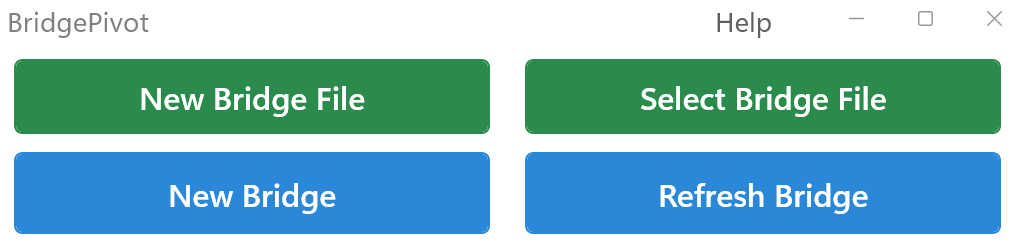
3.1 New Bridge button - Generates new dropdown menus and Bridge worksheets and other analysis frameworks Baselined on the Data worksheet data for subsequent data analysis. (Note: Related worksheets such as Bridge worksheets and corresponding data in the original workbook will be deleted.) If there are any changes to the Data worksheet data, you must first click the "New Bridge" button to generate a new analysis framework, then: 1. Make selections in the new Baseline and Comparison dropdown menus; 2. Click the "Refresh Bridge" button to regenerate the required Bridge charts and Contribution Analysis.
3.2 Refresh Bridge button - After selecting options in the Baseline and Comparison dropdown menus according to analysis needs, click the "Refresh Bridge" button to generate the required Bridge charts and Contribution Analysis. Missing data or worksheets will trigger prompts; it's recommended to click New Bridge to regenerate a new Bridge.
The dropdown menu is divided into two areas: Baseline and Comparison
The fields in Baseline and Comparison dropdown menus contain exactly the same options. Users can filter which options serve as Baseline data and which serve as Comparison data in the dropdown menus, using these as the comparison and analysis data for both ends of the Bridge. Note: Initially, by default, all fields in the Baseline and Comparison dropdown menus are selected, so Baseline and Comparison get exactly the same dataset, resulting in a Bridge with no differences.
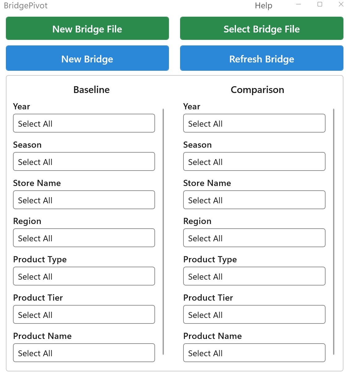
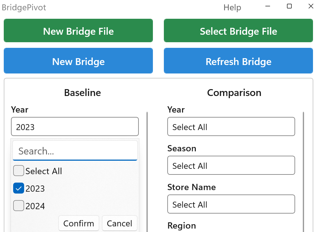
4.1 Baseline dropdown menu - Select the baseline data for comparison analysis. For example, we often use data from certain years as the comparison baseline, so here we select 2023.
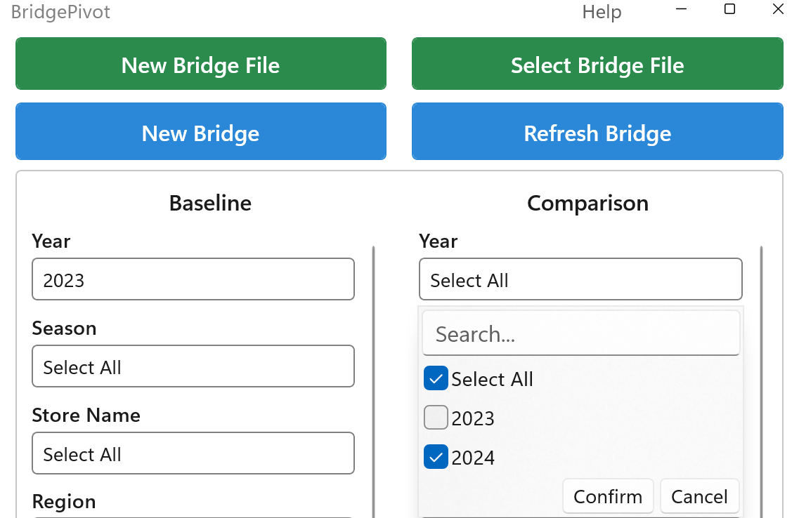
4.2 Comparison dropdown menu - Select the Comparison data for comparison analysis. For example, here we select 2024 as the year of interest to compare with 2023.
The Bridge worksheet displays the final analysis results, including Bridge charts and Contribution Analysis tables.
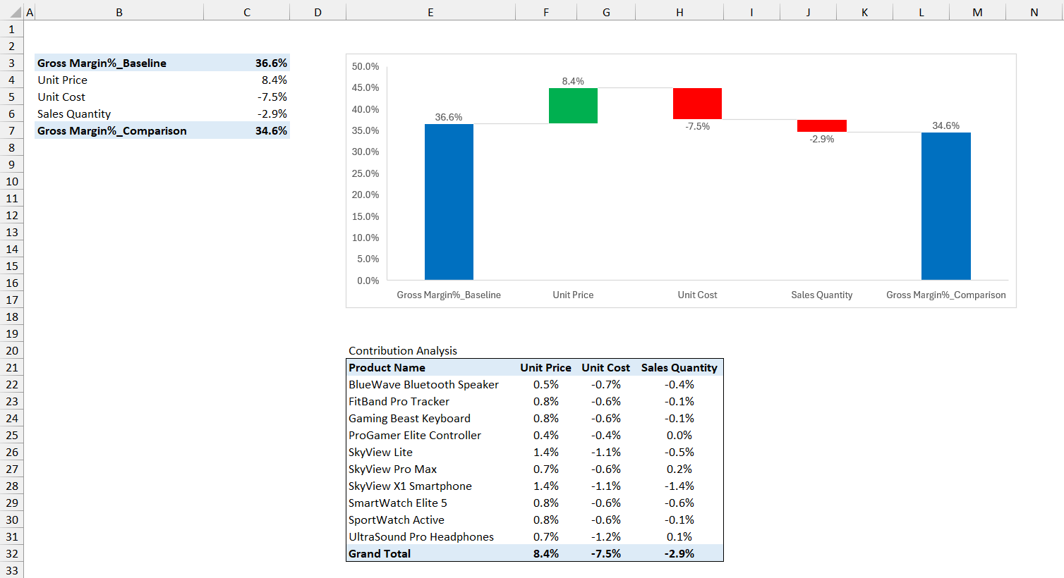
5.1 Bridge Data Source - Starting from cell B3 in the upper left corner, field names and data will appear. This is the data used to generate Bridge charts.
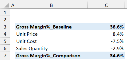
5.2 Bridge Chart - Displays the Bridge analyzed and obtained after program execution. The blue bar on the left is Baseline, the middle shows the impact contributed by each variable, and the right bar is Comparison.
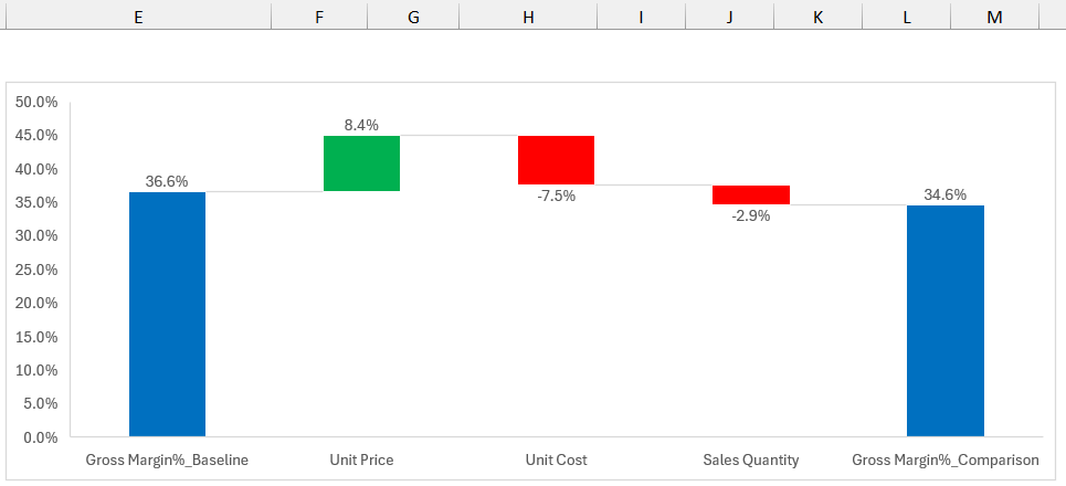
5.3 Contribution Analysis Table - Directly below the Bridge chart, a Contribution Analysis table will be displayed, showing the contribution of each Item in the Key field to overall changes under different factors.
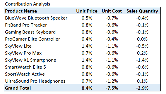
Through the Bridge Chart and Contribution Analysis Table, you can quickly identify the main Items (SKUs) affecting changes and the factors causing changes (price? cost? or quantity mix?).
You can analyze different dimensions and different result data by modifying 2.1 Data Type Selection to choose which field is Key and which field is Result. You can also use the dropdown menus to filter which data serves as Baseline and Comparison, then click Refresh Bridge to generate updated Bridge charts and Contribution Analysis tables for analyzing actual business situations and proposing improvement suggestions.
6. SumY and SumN Calculation Rules
Show the SumY / SumN calculation rules
In the first row Data Type of the Data worksheet, numerical values are divided into two types: SumY and SumN, and are used in formulas in the Result column. To correctly analyze the data, we define some calculation rules for SumY and SumN:
SumY + SumY = SumY
SumY + SumN (will show error)
SumN + SumN = SumN
SumY * SumY = SumY
SumY * SumN = SumY
SumN * SumN = SumN
SumY / SumY = SumN
SumY / SumN = SumY
SumN / SumY = SumN
SumN / SumN = SumN
Use Same Formula for Each Column: The program will automatically copy the formula from the fourth row to the entire column after removing fixed cell reference symbols "$" to ensure all formulas in each column are identical.
6.4.1 In formulas, if parentheses are included, calculations inside parentheses are performed first according to the order of operations, and the result is used as a value to continue calculations using the above rules.
Example: (SumY + SumY) * SumN
Step 1: SumY + SumY = SumY
Step 2: SumY * SumN = SumY
Final result type: SumY
6.4.2 If the Result column formula references other cells that also contain formulas, the analysis will merge all nested formulas into one formula for analysis.
Example:
Column E formula: =B*C (Total Cost = Quantity * Unit Cost)
Column F Result formula: =D-E (Profit = Revenue - Total Cost)
After merging: The program will analyze =D-(B*C)
6.4.3 The program will automatically reorder variables and apply the distributive property based on formula structure for better data analysis.
Original formula: =SumY*(SumN1 + SumN2)
After processing: =SumY*SumN1 + SumY*SumN2
This helps analyze the individual contributions of SumY, SumN1, and SumN2 more clearly.
7. Added Data and Removed Data
Show how Added / Removed data is handled
In real business scenarios, the items being compared between two periods are rarely identical. New products are launched, old products are discontinued, customers come and go, regions open and close. Bridge Analysis handles these structural changes through two dedicated concepts: Added Data and Removed Data.
Added Data — Records that exist in the Comparison period but did NOT exist in the Baseline period. They represent things that are entirely new, such as a newly launched product line, a newly opened store, or a newly acquired customer.
Removed Data — Records that existed in the Baseline period but NO LONGER exist in the Comparison period. They represent things that have been retired, discontinued, lost, or closed.
Because there is no "before" value for Added Data and no "after" value for Removed Data, their impact cannot be attributed to any single factor (such as price change, quantity change, or cost change). They must be isolated and reported on their own bars in the Bridge chart.
If Added Data and Removed Data are mixed into the regular price / quantity / mix variance calculations, the results become mathematically meaningless:
- A newly launched product has no Baseline price, so "price variance" is undefined.
- A discontinued product has no Comparison quantity, so "volume variance" is undefined.
- Forcing zero values into the formula would arbitrarily inflate or deflate other factors, distorting the entire bridge.
By isolating these two categories first, the remaining "like-for-like" items can be analyzed cleanly by price, volume, mix, cost, FX, and other true drivers.
The most common real-world manifestation of Added / Removed Data is the NPI / EOL product lifecycle:
- NPI — New Product Introduction: A product that just entered the market this year (Comparison) but did not exist last year (Baseline). Its entire revenue, cost, and margin are attributed to the Added Data bar.
- EOL — End of Life: A product that was sold last year (Baseline) but has been discontinued and removed from the catalog this year (Comparison). Its lost revenue and margin are attributed to the Removed Data bar.
The same pattern applies to many other business contexts:
- Retail / Store Network: Newly opened stores = Added Data; closed stores = Removed Data.
- Customer / Subscription Business: New customers acquired this period = Added Data; churned customers = Removed Data.
- Geographic Expansion: Newly entered countries / regions = Added Data; exited markets = Removed Data.
- M&A Activity: Acquired business units = Added Data; divested business units = Removed Data.
- Headcount Analysis: New hires = Added Data; departures = Removed Data.
Suppose a company is analyzing the year-over-year change in total revenue:
Baseline (2024) — Products A, B, C
- Product A: revenue 1,000
- Product B: revenue 800
- Product C (EOL — discontinued in 2025): revenue 300
- Baseline total: 2,100
Comparison (2025) — Products A, B, D
- Product A: revenue 1,100 (price + volume changes)
- Product B: revenue 900 (price + volume changes)
- Product D (NPI — launched in 2025): revenue 250
- Comparison total: 2,250
Bridge decomposition (Baseline 2,100 → Comparison 2,250, Δ = +150):
- Removed Data (Product C, EOL): −300
- Added Data (Product D, NPI): +250
- Like-for-like price / volume / mix change on A & B: +200
- Total change: −300 + 250 + 200 = +150 ✓
In the Bridge chart, the EOL impact and NPI impact appear as two clearly separated bars, while the remaining bars (price, volume, mix, etc.) reflect only the genuine performance change of products that exist in both periods. This makes the story easy to tell: "We lost 300 from EOL, gained 250 from NPI, and our existing portfolio grew by 200."
The program automatically detects Added and Removed records by comparing the Key columns (e.g., Product ID, Customer ID, Store ID) between the Baseline and Comparison data tables:
- A Key value that appears only in the Comparison table is treated as Added Data.
- A Key value that appears only in the Baseline table is treated as Removed Data.
- A Key value that appears in both tables is analyzed through normal factor decomposition (price, volume, cost, etc.).
No manual tagging is required — simply ensure your Key columns (such as Product Code) are consistent across both periods, and Bridge Analysis will handle NPI / EOL and similar structural changes correctly.
8. Other Worksheets
For the correct operation of the program, some other worksheets will be generated but hidden. Please do not modify these worksheets.
9. Data Security Assurance
Desktop Version (Use with Excel): All data exists only in local Excel files. The program runs entirely on your machine with no network communication during the analysis process.
Online Version (Use Online): Your spreadsheet data stays in your browser. Only a very small number of lightweight algorithm API requests are made to perform the Bridge calculation, and no user data is stored on our servers.
10. Transparent & Explainable Analysis
Reject the ambiguous conclusions and inexplicability of AI analysis. The analysis calculation process is completely transparent and explainable.
Process Worksheet Transparency
Contains the logic and algorithms for generating Bridge charts and data. Every calculation step can be traced and verified.
Traditional Black Box Analysis:
❌ "AI model shows 7pt profit margin decline"
❌ Cannot explain specific calculation process
❌ Cannot verify result accuracy
Bridge Transparent Analysis:
✅ "Price factor: -3pt, Cost factor: -2pt, Quantity factor: -2pt"
✅ Every calculation step visible in Process worksheet
✅ All formulas and logic completely verifiable
Local Data Security
Desktop Version: Zero network communication — all data processing completed locally, ensuring absolute enterprise data security.
Online Version: Only a very small number of lightweight algorithm API requests are made; no user data is stored on our servers.
Desktop Version (Use with Excel):
✅ Data never leaves your local computer
✅ No need to upload to cloud servers
✅ No network connection required during analysis
✅ Complies with strict enterprise data security policies
✅ Avoids data breach risks
Online Version (Use Online):
✅ Spreadsheet data stays in your browser
✅ Only a very small number of lightweight algorithm API requests are made
✅ No user data is stored on our servers
✅ Suitable for non-sensitive datasets and quick web-based analysis
Precise Mathematical Calculation
Based on rigorous mathematical formulas, ensuring accuracy and reliability of analysis results.
Traditional Estimation Analysis:
❌ Manual estimation with potential errors
❌ Cannot precisely quantify impact of each factor
❌ Aggregated results require manual adjustment
Bridge Precise Calculation:
✅ Mathematical formulas guarantee 100% accuracy
✅ Each factor's contribution precise to decimal places
✅ Totals automatically balance, no adjustment needed
Efficient Analysis
Complete complex analysis that traditionally takes days in just minutes, dramatically improving work efficiency.
Multi-dimensional Analysis
Support in-depth driving factor analysis by product, region, time, and other dimensions.
Flexible Configuration
Adjust analysis dimensions and comparison scenarios anytime to meet various business analysis needs.
Edit & Analyze in One Place — Built for Planning
Most tools only analyze data after it's finished. WaterfallBridge is different: a free, fully-featured online spreadsheet that runs on any platform. Upload your data — it stays in your browser — edit it live, and run driver & variance analysis instantly, with no export/import round trips.
Made for budgeting, forecasting & planning teams: change an assumption, see exactly what drives the gap, pinpoint the problem, and feed that insight straight back into your plan — for tighter, more accurate, defensible numbers.
Traditional Workflow:
❌ Build plan in one tool, export, re-import into an analysis tool
❌ Analysis is a separate, after-the-fact step
❌ Slow feedback loop — hard to test "what if" quickly
WaterfallBridge Closed Loop:
✅ Edit budget / forecast data right in the online sheet
✅ Instantly see which drivers move the result
✅ Adjust the plan and re-analyze in seconds — all in one place
✅ Free, cross-platform, and your data stays in your browser